Screening

By default pyTDGL assumes that screening is negligible, i.e., that the total vector potential in the film is equal to the applied vector potential: \(\mathbf{A}(\mathbf{r}, t)=\mathbf{A}_\mathrm{applied}(\mathbf{r}, t)\). Screening can optionally be included by evaluating the vector potential induced by currents flowing in the film. The vector potential in a 2D film induced by a sheet current density \(\mathbf{K}\) flowing in the film is given by

\[\mathbf{A}_\mathrm{induced}(\mathbf{r}, t) = \frac{\mu_0}{4\pi}\int_\mathrm{film}\frac{\mathbf{K}(\mathbf{r}', t)}{|\mathbf{r}-\mathbf{r}'|}\,\mathrm{d}^2\mathbf{r}'.\]

Taking the induced vector potential into account, the total vector potential in the film is \(\mathbf{A}(\mathbf{r}, t)=\mathbf{A}_\mathrm{applied}(\mathbf{r}, t)+\mathbf{A}_\mathrm{induced}(\mathbf{r}, t).\)

Because \(\mathbf{A} =\mathbf{A}_\mathrm{applied}+\mathbf{A}_\mathrm{induced}\) enters into the covariant gradient and Laplacian of \(\psi\), which in turn determine the current density \(\mathbf{J}=\mathbf{K}/d\), which determines \(\mathbf{A}_\mathrm{induced}\), the system must be solved self-consistently at each time step \(t^n\). The strategy for updating the induced vector potential to converge to a self-consistent value is based on Polyak’s “heavy ball” method:

\[\begin{split}\begin{split} \mathbf{A}^{n,s}_{\mathrm{induced},ij} &= \frac{\mu_0}{4\pi}\sum_{\text{sites } \ell}\frac{\mathbf{K}^{n,s}_\ell}{|\mathbf{r}_{ij}-\mathbf{r}_\ell|}a_\ell\\ \mathbf{d}^{n,s}_{ij} &= \mathbf{A}^{n,s}_{\mathrm{induced},ij} - \mathbf{A}^{n,s-1}_{\mathrm{induced},ij}\\ \mathbf{v}^{n,s+1} &= (1-\beta)\mathbf{v}^{n,s} + \alpha\mathbf{d}^{n,s}_{ij}\\ \mathbf{A}^{n,s+1}_{\mathrm{induced},ij} &= \mathbf{A}^{n,s}_{\mathrm{induced},ij} + \mathbf{v}^{n,s+1}_{ij} \end{split}\end{split}\]

The integer index \(s\) counts the number of iterations performed in the self-consistent calculation. The parameters \(\alpha\in(0,\infty)\) (the screening_step_size) and \(\beta\in(0,1)\) (the screening_drag) can be set by the user, and the initial conditions for \(\mathbf{A}^{n,0}_{\mathrm{induced},ij} = \mathbf{A}^{n-1}_{\mathrm{induced},ij}\) and \(\mathbf{v}^{n,0}_{ij} = \mathbf{0}\). The iterative application of the above equation terminates when the relative change in the induced vector potential between iterations falls below a user-defined tolerance (the screening_tolerance). The screening_step_size \(\alpha\) and screening_drag \(\beta\) determine the rate of convergence to the screening_tolerance.

In the equation above, we evaluate the sheet current density \(\mathbf{K}^n_\ell=\mathbf{K}(\mathbf{r}_\ell,t^n)\) on the mesh sites \(\mathbf{r}_\ell\) and the vector potential on the mesh edges \(\mathbf{r}_{ij}\), so the denominator \(|\mathbf{r}_{ij}-\mathbf{r}_\ell|\) is strictly greater than zero and the equation is well-defined. This method involves the pairwise distances between all edges and all sites in the mesh, so, in contrast to the sparse finite volume calculation, it is a “dense” problem. This means that including screening significantly increases the number of floating point operations required for a TDGL simulation.

A simple way to determine whether screening is non-negligible for a given model is to evaluate the fluxoid for a region inside a film for a small applied field, where the normalized order parameter \(\psi(\mathbf{r})=1\) everywhere. In this regime, the total fluxoid for a region containing no vortices should exactly vanish, as predicted by the London model. A fluxoid that differs significantly from zero when the model is solved without screening therefore indicates that screening should not be neglected, as demonstrated below.

[1]:

# Automatically install tdgl from GitHub only if running in Google Colab
if "google.colab" in str(get_ipython()):
    %pip install --quiet git+https://github.com/loganbvh/py-tdgl.git

[2]:

%config InlineBackend.figure_formats = {"retina", "png"}

import os
os.environ["OPENBLAS_NUM_THREADS"] = "1"

import matplotlib.pyplot as plt
import numpy as np

plt.rcParams["figure.figsize"] = (7.5, 2.5)

import tdgl
from tdgl.geometry import box, circle

Defining the device

Here we define a film with effective magnetic screening length \(\Lambda=\lambda^2/d=(0.075\,\mu\mathrm{m})^2 / (0.05\,\mu\mathrm{m})=0.1125\,\mu\mathrm{m}\), which is much smaller than the dimensions of the sample. We therefore expect screening to be important for this model.

[3]:

length_units = "um"
xi = 0.1
london_lambda = 0.075
thickness = 0.05

height = 1
width = 2

layer = tdgl.Layer(coherence_length=xi, london_lambda=london_lambda, thickness=thickness)
film = tdgl.Polygon("film", points=tdgl.geometry.box(width, height, points=301))
device = tdgl.Device(
    "bar",
    layer=layer,
    film=film,
    length_units=length_units,
)

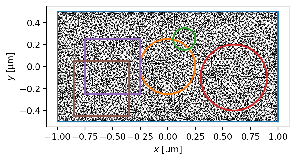
fluxoid_curves = [
    circle(0.25, center=(0, 0)),
    circle(0.1, center=(0.15, 0.25)),
    circle(0.3, center=(0.6, -0.1)),
    box(0.5, center=(-0.5, 0)),
    box(0.5, center=(-0.6, -0.2)),
]

[4]:

device.make_mesh(max_edge_length=xi / 2, smooth=100)

Constructing Voronoi polygons: 100%|███████████████████████████████████████████████████████████████████| 2862/2862 [00:00<00:00, 22832.46it/s]

[5]:

fig, ax = device.plot(mesh=True, legend=False)
for curve in fluxoid_curves:
    ax.plot(*curve.T, lw=2)

[6]:

device.mesh_stats()

[6]:

Mesh Statistics

num_sites	2862
num_elements	5426
min_edge_length	1.285e-02
max_edge_length	4.828e-02
mean_edge_length	2.896e-02
min_area	9.328e-05
max_area	1.446e-03
mean_area	6.988e-04
coherence_length	1.000e-01
length_units	um

Solve the model

Without screening

[7]:

options = tdgl.SolverOptions(
    solve_time=5,
    field_units="mT",
    current_units="uA",
    include_screening=False,
)

no_screening_solution = tdgl.solve(device, options, applied_vector_potential=0.1)

Simulating: 100%|████████████████████████████████████████████████████████████████████████████████████████████▊| 5/5 [00:00<00:00, 10.05tau/s ]

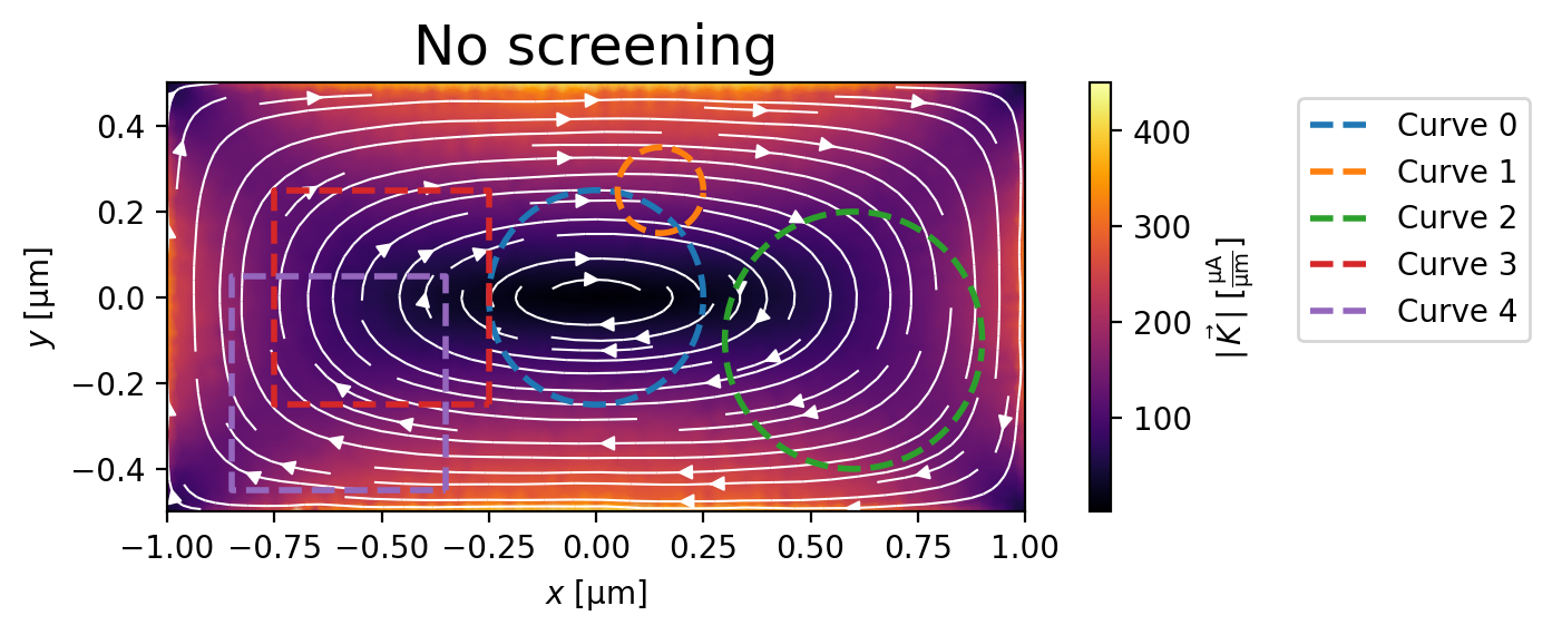
When screening is neglected, the Meissner supercurrent density is larger than predicted by London theory, meaning that the total vector potential \(\mathbf{A}\) and supercurrent density \(\mathbf{J}_s\) are not consistent, leading to a nonzero fluxoid \(\Phi_C\) for curve \(C\). In other words, the supercurrent does not “know” that some of the applied magnetic field should have been screened via the Meissner effect, so the supercurrent is responding to a larger magnetic field than would be present in a self-consistent scenario. We can quantify the error in the fluxoid by the ratio

\[\begin{split}\begin{split} \Phi_C &= \Phi_C^\mathrm{flux} + \Phi_C^\mathrm{supercurrent}\\ &= \oint_C\mathbf{A}(\mathbf{r})\cdot\mathrm{d}\mathbf{r} +\oint_C\mu_0\Lambda(\mathbf{r})\mathbf{K}_s(\mathbf{r})\cdot\mathrm{d}\mathbf{r}\\ \text{error}&=\left|\frac{\Phi_C^\mathrm{flux} + \Phi_C^\mathrm{supercurrent}}{\Phi_C^\mathrm{flux}}\right|. \end{split}\end{split}\]

[8]:

K = no_screening_solution.current_density
K_max = np.sqrt(K[:, 0]**2 + K[:, 1]**2).max()
print(f"Maximum sheet current density: {K_max:.1f~P}")

fig, ax = no_screening_solution.plot_currents()
_ = ax.set_title("No screening", fontsize=18)
for i, curve in enumerate(fluxoid_curves):
    fluxoid = no_screening_solution.polygon_fluxoid(curve)
    total_fluxoid = sum(fluxoid).magnitude
    error = abs(total_fluxoid / fluxoid.flux_part.magnitude)
    print(f"Curve {i}: total fluxoid {sum(fluxoid):.3e}, (error {100* error:.1f}%)")
    ax.plot(*curve.T, "--", lw=2, label=f"Curve {i}")

_ = ax.legend(bbox_to_anchor=(1.3, 1), loc="upper left")

Maximum sheet current density: 449.9 µA/µm

OMP: Info #276: omp_set_nested routine deprecated, please use omp_set_max_active_levels instead.

Curve 0: total fluxoid -1.260e-02 magnetic_flux_quantum, (error 392.6%)
Curve 1: total fluxoid -1.605e-03 magnetic_flux_quantum, (error 1307.5%)
Curve 2: total fluxoid -1.356e-02 magnetic_flux_quantum, (error 8524.0%)
Curve 3: total fluxoid -1.403e-02 magnetic_flux_quantum, (error 651.0%)
Curve 4: total fluxoid -1.019e-02 magnetic_flux_quantum, (error 619.7%)

With screening

[9]:

options = tdgl.SolverOptions(
    solve_time=5,
    field_units="mT",
    current_units="uA",
    include_screening=True,
    screening_tolerance=1e-6,
    dt_max=1e-3,
)

screening_solution = tdgl.solve(device, options, applied_vector_potential=0.1)

Simulating: 100%|████████████████████████████████████████████████████████████████████████████████████████████▉| 5/5 [00:55<00:00, 11.17s/tau ]

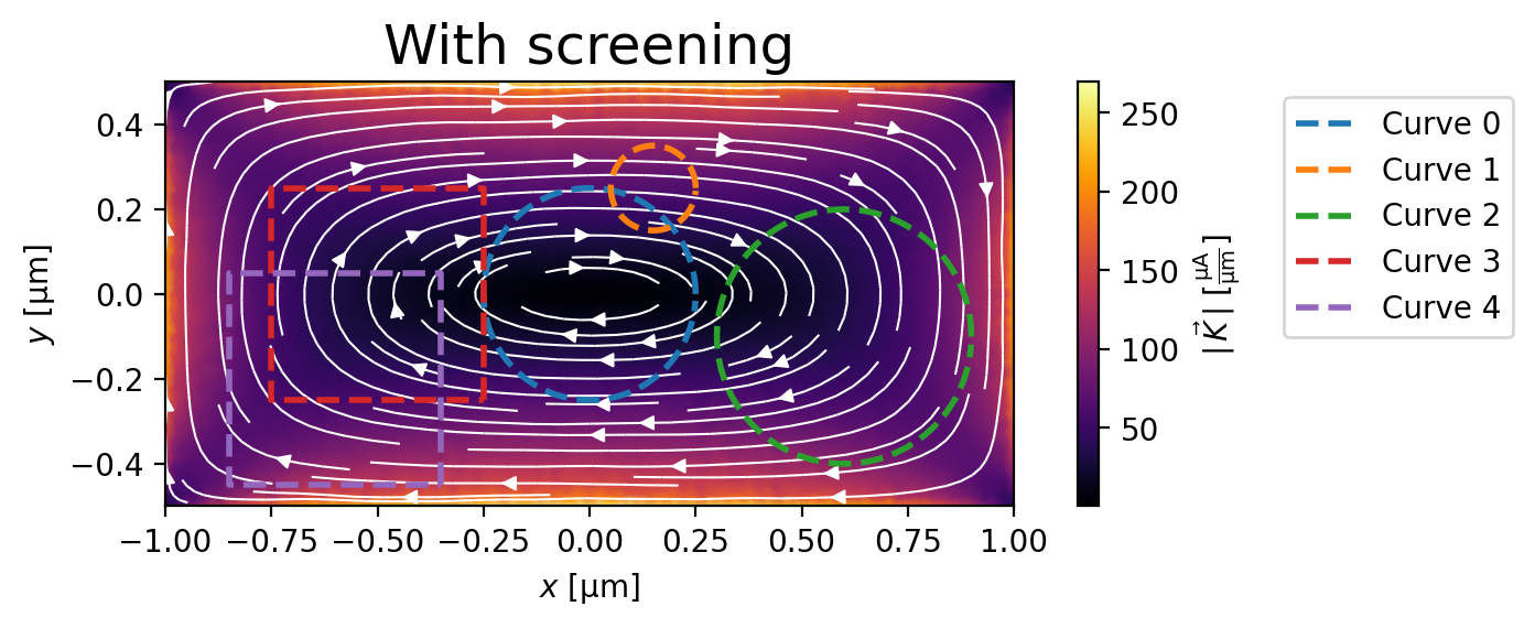
When screening is included, the supercurrent density is smaller and the fluxoid \(\Phi_C\) is quantized at 0 \(\Phi_0\) to within a few percent.

[10]:

K = screening_solution.current_density
K_max = np.sqrt(K[:, 0]**2 + K[:, 1]**2).max()
print(f"Maximum sheet current density: {K_max:.1f~P}")

fig, ax = screening_solution.plot_currents()
_ = ax.set_title("With screening", fontsize=18)

for i, curve in enumerate(fluxoid_curves):
    ax.plot(*curve.T, "--", lw=2, label=f"Curve {i}")
    fluxoid = screening_solution.polygon_fluxoid(curve)
    total_fluxoid = sum(fluxoid).magnitude
    error = abs(total_fluxoid / fluxoid.flux_part.magnitude)
    print(f"Curve {i}: total fluxoid {sum(fluxoid):.3e}, (error {100 * error:.1f}%)")

_ = ax.legend(bbox_to_anchor=(1.3, 1), loc="upper left")

Maximum sheet current density: 269.5 µA/µm
Curve 0: total fluxoid -7.348e-05 magnetic_flux_quantum, (error 2.0%)
Curve 1: total fluxoid -2.530e-05 magnetic_flux_quantum, (error 3.6%)
Curve 2: total fluxoid -3.784e-05 magnetic_flux_quantum, (error 0.6%)
Curve 3: total fluxoid -5.936e-05 magnetic_flux_quantum, (error 1.1%)
Curve 4: total fluxoid 5.292e-05 magnetic_flux_quantum, (error 0.8%)

[11]:

tdgl.version_table()

[11]:

Software	Version
tdgl	0.8.1; git revision 25e009d [2024-04-10]
Numpy	1.24.3
SciPy	1.10.1
matplotlib	3.7.1
cupy	None
numba	0.57.1
IPython	8.14.0
Python	3.10.11 \| packaged by conda-forge \| (main, May 10 2023, 19:01:19) [Clang 14.0.6 ]
OS	posix [darwin]
Number of CPUs	Physical: 10, Logical: 10
BLAS Info	OPENBLAS
Wed Apr 10 14:05:16 2024 PDT

[ ]: