Theoretical Background
Tip
pyTDGL is described in detail in the following paper:
pyTDGL: Time-dependent Ginzburg-Landau in Python, Computer Physics Communications 291, 108799 (2023), DOI: 10.1016/j.cpc.2023.108799.
The accepted version of the paper can also be found on arXiv: arXiv:2302.03812.
Here we sketch out the generalized time-dependent Ginzburg-Landau model implemented in pyTDGL, and the numerical methods used to solve it.
This material and portions of the pyTDGL package are based on Refs. [1][2] (repo). The generalized
time-dependent Ginzburg-Landau theory is based on Refs. [3][4]. The numerical methods are based on
Refs. [1][5][6].
pyTDGL can model superconducting thin films of arbitrary geometry, including multiply-connected films (i.e., films with holes).
By “thin” or “two-dimensional” we mean that the film thickness \(d\) is smaller than the coherence length \(\xi=\xi(T)\)
and the London penetration depth \(\lambda=\lambda(T)\), where \(T\) is temperature. This assumption implies that both the
superconducting order parameter \(\psi(\mathbf{r})\) and the supercurrent \(\mathbf{J}_s(\mathbf{r})\) are roughly
constant over the thickness of the film.
Strictly speaking, the model is only valid for temperatures very close to the critical
temperature, \(T/T_c\approx 1\), and for dirty superconductors where the inelastic diffusion length much smaller than the
coherence length \(\xi\) [3].
Time-dependent Ginzburg-Landau
The time-dependent Ginzburg-Landau formalism employed here [3] boils down to a set of coupled partial differential equations for a complex-valued field \(\psi(\mathbf{r}, t)=|\psi|e^{i\theta}\) (the superconducting order parameter) and a real-valued field \(\mu(\mathbf{r}, t)\) (the electric scalar potential), which evolve deterministically in time for a given time-independent applied magnetic vector potential \(\mathbf{A}(\mathbf{r})\).
The order parameter \(\psi\) evolves according to:
The quantity \((\nabla-i\mathbf{A})^2\psi\) is the covariant Laplacian of \(\psi\), which is used in place of an ordinary Laplacian in order to maintain gauge-invariance of the order parameter. Similarly, \((\frac{\partial}{\partial t}+i\mu)\psi\) is the covariant time derivative of \(\psi\). \(u=\pi^4/(14\zeta(3))\approx5.79\) is the ratio of relaxation times for the amplitude and phase of the order parameter in dirty superconductors (\(\zeta\) is the Riemann zeta function) and \(\gamma\) is a material parameter which is proportional to the inelastic scattering time and the size of the superconducting gap. \(\epsilon(\mathbf{r})=T_c(\mathbf{r})/T - 1 \in [-1,1]\) is a real-valued parameter that adjusts the local critical temperature of the film. Setting \(\epsilon(\mathbf{r}) < 1\) suppresses the critical temperature at position \(\mathbf{r}\), and extended regions of \(\epsilon(\mathbf{r}) < 0\) can be used to model large-scale metallic pinning sites [7][8][9].
The electric scalar potential \(\mu(\mathbf{r}, t)\) evolves according to the Poisson equation:
where \(\mathbf{J}_s=\mathrm{Im}[\psi^*(\nabla-i\mathbf{A})\psi]\) is the supercurrent density. Again, \((\nabla-i\mathbf{A})\psi\) is the covariant gradient of \(\psi\).
In addition to the electric potential (Eq. 2), one can couple the dynamics of the order parameter (Eq. 1) to other physical quantities to create a “multiphysics” model. For example, it is common to couple the TDGL equations to the local temperature \(T(\mathbf{r}, t)\) of the superconductor via a heat balance equation to model self-heating [10][11][12][13][14].
Boundary conditions
Isolating boundary conditions are enforced on superconductor-vacuum interfaces, in form of Neumann boundary conditions for \(\psi\) and \(\mu\):
Superconductor-normal metal interfaces can be used to apply a bias current density \(J_\mathrm{ext}\). For such interfaces, we impose Dirichlet boundary conditions on \(\psi\) and Neumann boundary conditions on \(\mu\):
A single model can have an arbitrary number of current terminals (although just 1 terminal is not allowed due to current conservation). If we label the terminals \(i=1,2,\ldots\), we can express the global current conservation constraint as
where \(I_{\mathrm{ext},i}\) is the total current through terminal \(i\), \(L_i\) is the length of terminal \(i\), and \(J_{\mathrm{ext},i}\) is the current density along terminal \(i\), which we assume to be constant and directed normal to the terminal. From Eq. 5, it follows that the current boundary condition for terminal \(i\) is:
Units
The TDGL model [Eq. 1, Eq. 2] is solved in dimensionless units, where the scale factors are given in terms of fundamental constants and material parameters, namely the superconducting coherence length \(\xi\), London penetration depth \(\lambda\), normal state conductivity \(\sigma\), and film thickness \(d\). The Ginzburg-Landau parameter is defined as \(\kappa=\lambda/\xi\). \(\mu_0\) is the vacuum permeability and \(\Phi_0=h/2e\) is the superconducting flux quantum.
Time is measured in units of \(\tau_0 = \mu_0\sigma\lambda^2\)
Magnetic field is measured in units of the upper critical field \(B_0=B_{c2}=\mu_0H_{c2} = \frac{\Phi_0}{2\pi\xi^2}\)
Magnetic vector potential is measured in units of \(A_0=\xi B_0=\frac{\Phi_0}{2\pi\xi}\)
Current density is measured in units of \(J_0=\frac{4\xi B_{c2}}{\mu_0\lambda^2}\)
Sheet current density is measured in units of \(K_0=J_0 d=\frac{4\xi B_{c2}}{\mu_0\Lambda}\), where \(\Lambda=\lambda^2/d\) is the effective magnetic penetration depth
Voltage is measured in units of \(V_0=\xi J_0/\sigma=\frac{4\xi^2 B_{c2}}{\mu_0\sigma\lambda^2}\)
Numerical implementation
Finite volume method
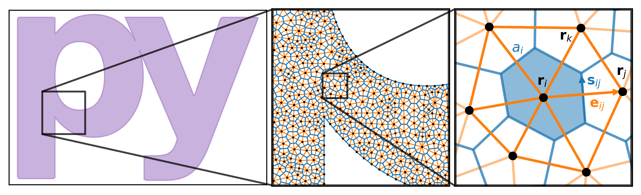
We solve the TDGL model [Eq. 1, Eq. 2] on an unstructured Delaunay mesh in two dimensions [6][1]. The mesh is composed of a set of sites, each denoted by its position \(\mathbf{r}_i\in\mathbb{R}^2\) or an integer index \(i\), and a set of triangular cells \(c_{ijk}\). Each cell \(c_{ijk}=(i, j, k)\) represents a triangle with three edges (\((i, j)\), \((j, k)\), and \((k, i)\)) that connect sites \(\mathbf{r}_i\), \(\mathbf{r}_j\), \(\mathbf{r}_k\) in a counterclockwise fashion. Each edge (denoted by the vector \(\mathbf{e}_{ij}=\mathbf{r}_j-\mathbf{r}_i\) or the 2-tuple \((i, j)\)) has a length \(e_{ij}=|\mathbf{e}_{ij}|\) and a direction \(\hat{\mathbf{e}}_{ij}=\mathbf{e}_{ij}/e_{ij}\). Each site is assigned an effective area \(a_i\), which is the area of the Voronoi region surrounding the site. The Voronoi region surrounding site \(i\) consists of all points in space that are closer to site \(\mathbf{r}_i\) than to any other site in the mesh. The side of the Voronoi region that intersects edge \((i, j)\) is denoted \(\mathbf{s}_{ij}\) and has a length \(s_{ij}\). The collection of all Voronoi cells tesselates the film and forms a mesh that is dual to the triangular Delaunay mesh.
A scalar function \(f(\mathbf{r}, t)\) can be discretized at a given time \(t^{n}\) as the value of the function on each site, \(f_i^{n}=f(\mathbf{r}_i, t^{n})\). A vector function \(\mathbf{F}(\mathbf{r}, t)\) can be discretized at time \(t^{n}\) as the flow of the vector field between sites. In other words, \(F_{ij}^{n}=\mathbf{F}((\mathbf{r}_i+\mathbf{r}_j)/2, t^{n})\cdot\hat{\mathbf{e}}_{ij}\), where \((\mathbf{r}_i+\mathbf{r}_j)/2=\mathbf{r}_{ij}\) is the center of edge \((i, j)\).
The gradient of a scalar function \(g(\mathbf{r})\) is approximated on the edges of the mesh. The value of \(\nabla g\) at position \(\mathbf{r}_{ij}\) (i.e., the center of edge \((i, j)\)) is:
To calculate the divergence of a vector field \(\mathbf{F}(\mathbf{r})\) on the mesh, we assume that each Voronoi cell is small enough that the value of \(\nabla\cdot\mathbf{F}\) is constant over the area of the cell and equal to the value at the mesh site lying inside the cell, \(\mathbf{r}_i\). Then, using the divergence theorem in two dimensions, we have
where \(\mathcal{N}(i)\) is the set of sites adjacent to site \(\mathbf{r}_i\).
The Laplacian of a scalar function \(g\) is given by \(\nabla^2 g=\nabla\cdot\nabla g\), so combining Eq. 7 and Eq. 8 we have
The discrete gradient, divergence, and Laplacian of a field at site \(i\) depend only on the value of the field at site \(i\) and its nearest neighbors. This means that the corresponding operators, Eq. 7, Eq. 8, and Eq. 9, can be represented efficiently as sparse matrices, and their action given by a matrix-vector product.
Covariant derivatives
We use link variables [5][6] to construct covariant versions of the spatial derivatives and time derivatives of \(\psi\). In the discrete case corresponding to our finite volume method, this amounts to adding a complex phase whenever taking a difference in \(\psi\) between mesh sites (for spatial derivatives) or time steps (for time derivatives).
The discretized form of the covariant gradient of \(\psi\) at time \(t^{n}\) and edge \(\mathbf{r}_{ij}\) is:
where \(U^{n}_{ij}=\exp(-i\mathbf{A}(\mathbf{r}_{ij}, t^{n})\cdot\mathbf{e}_{ij}) = \exp(-iA_{ij}e_{ij})^{n}\) is the spatial link variable. Eq. 10 is similar to the gauge-invariant phase difference in Josephson junction physics.
The discretized form of the covariant Laplacian of \(\psi\) at time \(t^{n}\) and site \(\mathbf{r}_i\) is:
The discretized form of the covariant time-derivative of \(\psi\) at time \(t^{n}\) and site \(\mathbf{r}_i\) is
where \(U_i^{n, n+1}=\exp(i\mu_i^{n}\Delta t^{n})\) is the temporal link variable.
Implicit Euler method
The discretized form of the equations of motion for \(\psi(\mathbf{r}, t)\) and \(\mu(\mathbf{r}, t)\) are given by
where \(A_{ij}^{n} = \mathbf{A}(\mathbf{r}_{ij}, t^{n})\cdot\hat{\mathbf{e}}_{ij}\) and \(\frac{A_{ij}^{n} - A_{ij}^{n-1}}{\Delta t^{n}}\) approximates the time derivative of the vector potential, \(\left.\partial\mathbf{A}/\partial t\right|_{\mathbf{r}_{ij}}^{t_n}\).
If we isloate the terms in Eq. 13 involving the order parameter at time \(t^{n+1}\), we can rewrite Eq. 13 in the form
where
and
Solving Eq. 15 for \(\left|\psi_i^{n+1}\right|^2\), we arrive at a quadratic equation in \(\left|\psi_i^{n+1}\right|^2\) (see Appendices for the full calculation):
where we have defined
To solve Eq. 18, which has the form \(0=ax^2+bx+c\), we use a modified quadratic formula:
in order to avoid numerical issues when \(a=\left|z_i^n\right|^2=0\), i.e., when \(\left|\psi_i^n\right|^2=0\) or \(\gamma=0\). Applying Eq. 19 to Eq. 18 yields
We take the root with the “\(+\)” sign in Eq. 20 because the “\(-\)” sign results in unphysical behavior where \(\left|\psi_i^{n+1}\right|^2\) diverges when \(\left|z_i^{n}\right|^2\) vanishes (i.e., when \(\left|\psi_i^{n}\right|^2\) is zero).
Combining Eq. 15 and Eq. 20 allows us to find the order parameter at time \(t^{n+1}\) in terms of the order parameter and scalar potential at time \(t^{n}\):
Combining Eq. 21 and Eq. 14 yields a sparse linear system that can be solved to find \(\mu_i^{n+1}\) given \(\mu_i^{n}\) and \(\psi_i^{(n + 1)}\). The Poisson equation, Eq. 14, is solved using sparse LU factorization [15].
Adaptive time step
pyTDGL implements an adaptive time step algorithm that adjusts the time step \(\Delta t^{n}\)
based on the speed of the system’s dynamics. This functionality is useful if, for example, you are only interested
in the equilibrium behavior of a system. The dynamics may initially be quite fast and then slow down as you approach steady state.
Using an adaptive time step dramatically reduces the wall-clock time needed to model equilibrium behavior in such instances, without
sacrificing solution accuracy.
There are four parameters that control the adaptive time step algorithm, which are defined in tdgl.SolverOptions:
\(\Delta t_\mathrm{init}\) (SolverOptions.dt_init),
\(\Delta t_\mathrm{max}\) (SolverOptions.dt_max),
and \(N_\mathrm{window}\) (SolverOptions.adaptive_window) \(M_\mathrm{adaptive}\) (SolverOptions.adaptive_time_step_multiplier).
The initial time step at iteration \(n=0\) is set to \(\Delta t^{(0)}=\Delta t_\mathrm{init}\). We keep a running list of
\(\Delta|\psi|^2_n=\max_i \left|\left(\left|\psi_i^{n}\right|^2-\left|\psi_i^{n-1}\right|^2\right)\right|\) for each iteration \(n\).
Then, for each iteration \(n > N_\mathrm{window}\), we define a tentative new time step \(\Delta t_\star\)
using the following heuristic:
Eq. 22 has the effect of automatically selecting a small time step if the recent dynamics of the order parameter are fast, and a larger time step if the dynamics are slow.
Note
Because new time steps are chosen based on the dynamics of the order parameter, we recommend disabling
the adaptive time step algorithm or using a strict \(\Delta t_\mathrm{max}\) in cases where the entire
superconductor is in the normal state, \(\psi=0\). You can use a fixed time step by setting
tdgl.SolverOptions(..., adaptive=False, ...).
The the time step selected at iteration \(n\) as described above may be too large to accurately solve for the state of the system in iteration \(m=n+1\). We detect such a failure to converge by evaluating the discriminant of Eq. 18. If the discriminant, \((2c_i^{m} + 1)^2 - 4|z_i^{m}|^2|w_i^{m}|^2\), is less than zero for any site \(i\), then the value of \(|\psi_i^{m+1}|^2\) found in Eq. 20 will be complex, which is unphysical. If this happens, we iteratively reduce the time step \(\Delta t^{m}\) (setting \(\Delta t^{m} \leftarrow \Delta t^{m}\times M_\mathrm{adaptive}\) at each iteration) and re-solve Eq. 18 until the discriminant is nonnegative for all sites \(i\), then proceed with the rest of the calculation for iteration \(m\).
Appendices
Implicit Euler method
Here we go through the full derivation of the quadratic equation for \(\left|\psi_i^{n+1}\right|^2\), Eq. 18, starting from Eq. 15:
Screening
By default pyTDGL assumes that screening is negligible, i.e., that the total vector potential in the film is
equal to the applied vector potential: \(\mathbf{A}(\mathbf{r}, t)=\mathbf{A}_\mathrm{applied}(\mathbf{r})\).
Screening can optionally be included by evaluating the vector potential induced by currents flowing in the film.
The vector potential in a 2D film induced by a sheet current density \(\mathbf{K}\) flowing in the film is given by
Taking the induced vector potential into account, the total vector potential in the film is
Because \(\mathbf{A} =\mathbf{A}_\mathrm{applied}+\mathbf{A}_\mathrm{induced}\) enters into the covariant gradient and Laplacian of \(\psi\) (Eq. 10 and Eq. 11), which in turn determine the current density \(\mathbf{J}=\mathbf{K}/d\), which determines \(\mathbf{A}_\mathrm{induced}\), Eq. 24 must be solved self-consistently at each time step \(t^n\). The strategy for updating the induced vector potential to converge to a self-consistent value is based on Polyak’s “heavy ball” method [16][17]:
The integer index \(s\) counts the number of iterations performed in the self-consistent calculation. The parameters \(\alpha\in(0,\infty)\) and \(\beta\in(0,1]\) in Eq. 26 can be set by the user, and the initial conditions for Eq. 26 are \(\mathbf{A}^{n,0}_{\mathrm{induced},ij} = \mathbf{A}^{n-1}_{\mathrm{induced},ij}\) and \(\mathbf{v}^{n,0}_{ij} = \mathbf{0}\). The iterative application of Eq. 26 terminates when the relative change in the induced vector potential between iterations falls below a user-defined tolerance.
In Eq. 26, we evaluate the sheet current density \(\mathbf{K}^n_\ell=\mathbf{K}(\mathbf{r}_\ell,t^n)\) on the mesh sites \(\mathbf{r}_\ell\), and the vector potential on the mesh edges \(\mathbf{r}_{ij}\), so the denominator \(|\mathbf{r}_{ij}-\mathbf{r}_\ell|\) is strictly greater than zero and Eq. 26 is well-defined. Eq. 26 involves the pairwise distances between all edges and all sites in the mesh, so, in contrast to the sparse finite volume calculation, it is a “dense” problem. This means that including screening significantly increases the number of floating point operations required for a TDGL simulation.
Pseduocode for the solver algorithms
Adaptive Euler update
Adaptive Euler update subroutine. The parameters \(M_\mathrm{adaptive}\) and \(N_\mathrm{retries}^\mathrm{max}\) can be set by the user.
Data: \(\psi_i^n\), \(\Delta t_\star\), \(M_\mathrm{adaptive}\), \(N_\mathrm{retries}^\mathrm{max}\)Result: \(\psi_i^{n+1}\), \(\Delta t^n\)
\(\Delta t^n \gets \Delta t_\star\)
Calculate \(z_i^n\), \(w_i^n\), \(\left|\psi_i^{n+1}\right|^2\) given \(\Delta t^n\) (Eq. 16, Eq. 17, Eq. 20)
if adaptive:
\(N_\mathrm{retries} \gets 0\)
while \(\left|\psi_i^{n+1}\right|^2\) is complex for any site \(i\):
if \(N_\mathrm{retries} > N_\mathrm{retries}^\mathrm{max}\):
Failed to converge - raise an error.
\(\Delta t^n \gets \Delta t^n \times M_\mathrm{adaptive}\)
Calculate \(z_i^n\), \(w_i^n\), \(\left|\psi_i^{n+1}\right|^2\) given \(\Delta t^n\) (Eq. 16, Eq. 17, Eq. 20)
\(N_\mathrm{retries} \gets N_\mathrm{retries} + 1\)
\(\psi_i^{n+1} \gets w_i^n - z_i^n \left|\psi_i^{n+1}\right|^2\) (Eq. 21)
Solve step, no screening
A single solve step, in which we solve for the state of the system at time \(t^{n+1}\) given the state of the system at time \(t^n\), with no screening.
Data: \(n\), \(t^n\), \(\Delta t_\star\), \(\psi_i^{n}\), \(\mu_i^{n}\)Result: \(t^{n+1}\), \(\Delta t^{n}\), \(\psi_i^{n+1}\), \(\mu_i^{n+1}\), \(J_{s,ij}^{n+1}\), \(J_{n,ij}^{n+1}\), \(\Delta t_\star\)
Evaluate current density \(J^{n+1}_{\mathrm{ext},\,k}\) for terminals \(k\) (Eq. 6)
Update boundary conditions for \(\mu_i^{n+1}\) (Eq. 4)
Calculate \(\psi_i^{n+1}\) and \(\Delta t^n\) via Adaptive Euler update
Calculate the supercurrent density \(J_{s,ij}^{n+1}\) (Eq. 14)
Solve for \(\mu_i^{n+1}\) via sparse LU factorization (Eq. 14)
Evaluate normal current density \(J_{n,ij}^{n+1}\) via \(\mathbf{J}_n=-\nabla\mu - \frac{\partial\mathbf{A}}{\partial t}\)
if adaptive:
Select new tentative time step \(\Delta t_\star\) given \(\Delta t^n\) (Eq. 22)
\(t^{n+1} \gets t^{n} + \Delta t^{n}\)
\(n \gets n + 1\)
Solve step, with screening
A single solve step, with screening. The parameters \(A_\mathrm{tol}\) and \(N_\mathrm{screening}^\mathrm{max}\) can be set by the user.
Data: \(n\), \(t^n\), \(\Delta t_\star\), \(\psi_i^{n}\), \(\mu_i^{n}\), \(\mathbf{A}^n_{\mathrm{induced}}\)Result: \(t^{n+1}\), \(\Delta t^{n}\), \(\psi_i^{n+1}\), \(\mu_i^{n+1}\), \(J_{s,ij}^{n+1}\), \(J_{n,ij}^{n+1}\), \(\mathbf{A}^{n+1}_{\mathrm{induced}}\), \(\Delta t_\star\)
Evaluate current density \(J^{n+1}_{\mathrm{ext},\,k}\) for terminals \(k\) (Eq. 6)
Update boundary conditions for \(\mu_i^{n+1}\) (Eq. 4)
\(s \gets 0\), screening iteration index
\(\mathbf{A}^{n+1,s}_\mathrm{induced} \gets \mathbf{A}^{n}_\mathrm{induced}\), initialize induced vector potential based on solution from previous time step
\(\delta A_\mathrm{induced} \gets \infty\), relative error in induced vector potential
while \(\delta A_\mathrm{induced} > A_\mathrm{tol}\):
if \(s > N_\mathrm{screening}^\mathrm{max}\):
Failed to converge - raise an error.
if \(s==0\):
\(\Delta t^n \gets \Delta t_\star\), initial guess for new time step
Update link variables in \((\nabla-i\mathbf{A})\) and \((\nabla -i\mathbf{A})^2\) given \(\mathbf{A}_\mathrm{induced}^{n+1,s}\) (Eq. 10, Eq. 11)
Calculate \(\psi_i^{n+1}\) and \(\Delta t^n\) via Adaptive Euler update
Calculate the supercurrent density \(J_{s,ij}^{n+1}\) (Eq. 14)
Solve for \(\mu_i^{n+1}\) via sparse LU factorization (Eq. 14)
Evaluate normal current density \(J_{n,ij}^{n+1}\) via \(\mathbf{J}_n=-\nabla\mu - \frac{\partial\mathbf{A}}{\partial t}\)
Evaluate \(\mathbf{K}_i^{n+1}=d(\mathbf{J}_{s,i}^{n+1}+\mathbf{J}_{n,i}^{n+1})\) at the mesh sites \(i\)
Update induced vector potential \(\mathbf{A}^{n+1,s}_\mathrm{induced}\) (Eq. 26)
if \(s > 1\):
\(\delta A_\mathrm{induced} \gets \max_\mathrm{edges}\left(\left|\mathbf{A}^{n+1,s}_\mathrm{induced}-\mathbf{A}^{n+1,s-1}_\mathrm{induced}\right|/\left|\mathbf{A}^{n+1,s}_\mathrm{induced}\right|\right)\)
\(s \gets s + 1\)
\(\mathbf{A}^{n+1}_\mathrm{induced} \gets \mathbf{A}^{n+1,s}_\mathrm{induced}\), self-consistent value of the induced vector potential
if adaptive:
Select new tentative time step \(\Delta t_\star\) (Eq. 22)
\(t^{n+1} \gets t^{n} + \Delta t^{n}\)
\(n \gets n + 1\)